Computing Set Relationships: The Containing Parents Approach

What Are Set Relationships?

Deliberate API uses Uber's H3 hexagonal hierarchical spatial index to represent geographic areas. Each "set" is a collection of H3 indexes that represents a geographic region—like a country, state, or custom user-defined area. As I worked through the build out of Deliberate API I came across the idea of relationships between sets. This was driven by the powerful hierachal structure that H3 provides. H3 indexes (hexagons) are organized into a hierarchical structure where each index is made up of 7 smaller hexagons. When you start defining sets using these h3 indexes you find yourself asking questions like "do the two sets I care about. Set A and set B share any hexagons?" or "is every h3 index in set A also in set B?". This lead to set relationships becoming first class citizens in Deliberate API.

Currently, Deliberate API supports two types of relationships between sets:

• Intersects - Set A and Set B share at least one H3 index
• Subset - Set A is contained within Set B (roughly 93% or more of Set A's indexes are in Set B)

Why 93% for subset detection?

I've always enjoyed math and the beauty of it. I also love a good mathematical definition, so it pains me that I use the word "subset" to describe a relationship that isn't truly a mathematical subset. However, when we're talking about geographic areas and H3 indexes, we run into some practical challenges.

Here's the problem:

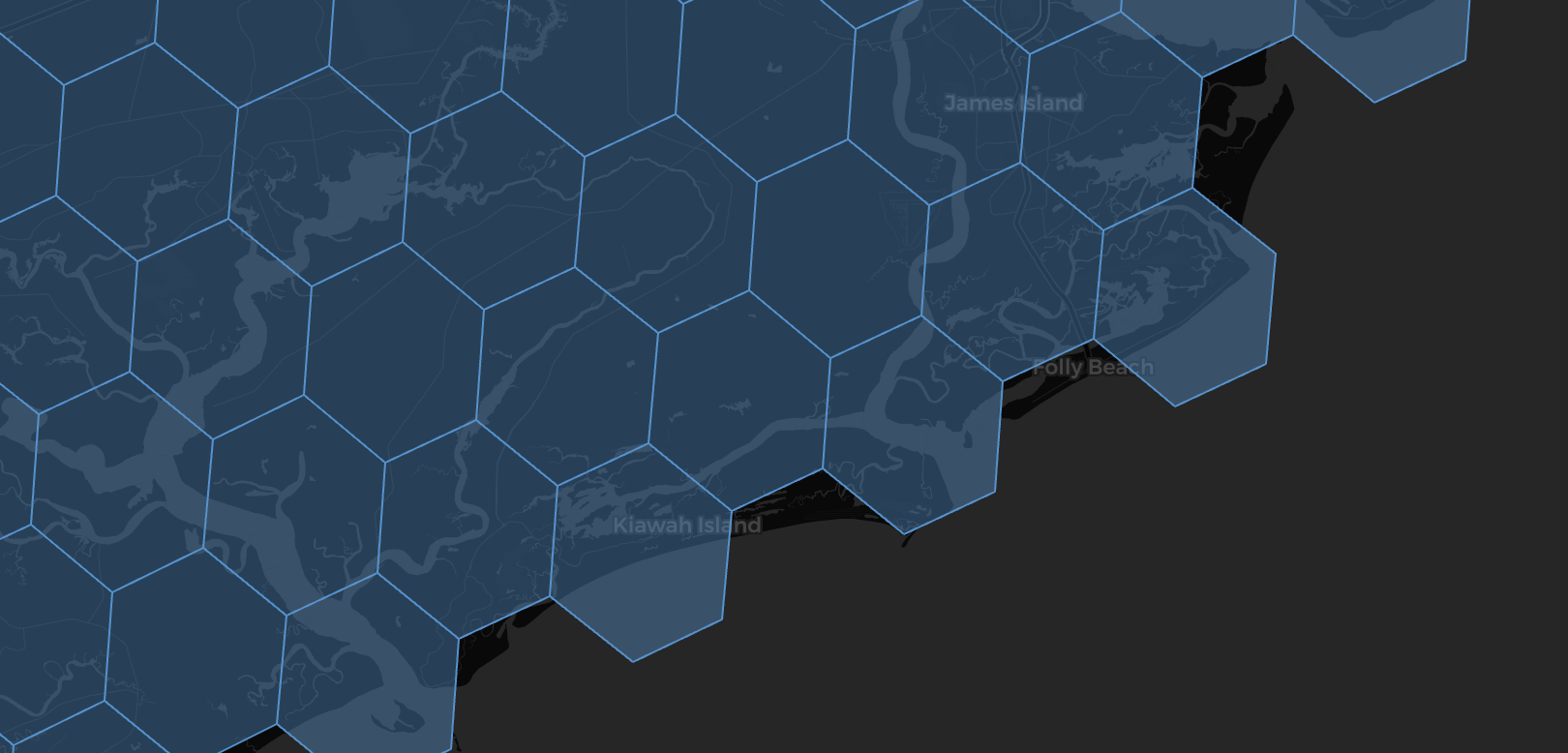
Figure 1: South Carolina at resolution 6 (2,527 hexagons) - notice the jagged edges

You see that we can't fully capture the perfect edges of a set. This is an artifact of optimization. We could increase the resolution of the H3 indexes we use to fill the set, which would give us much prettier edges. For example, let's bump up one resolution and see what happens:

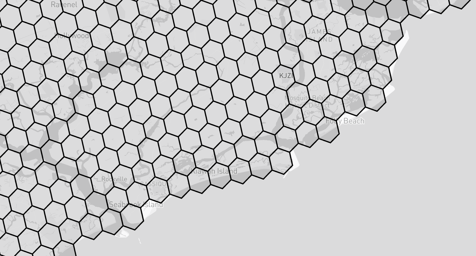
Figure 2: South Carolina at resolution 7 (17,632 hexagons) - smoother, but at what cost?

Immediately you can see the tradeoff: we jumped from 2,527 hexagons at resolution 6 to 17,632 hexagons at resolution 7. That's 7× more indexes to store, query, and compute relationships for.

I've found that getting a pretty edge is not worth the extra compute that comes with the larger set of indexes. So we accept a loss of precision around the edges to gain the benefit of a smaller, more manageable set of indexes.

Why do we lose hexagons at the edges?

H3's polygon fill algorithm includes a hexagon if its center point falls inside the polygon. Edge hexagons where the center happens to fall just outside get excluded.

Now here's where this becomes a problem for subset detection. When we look at the relationship between Set A (South Carolina) and Set B (the United States), those jagged edges create gaps:

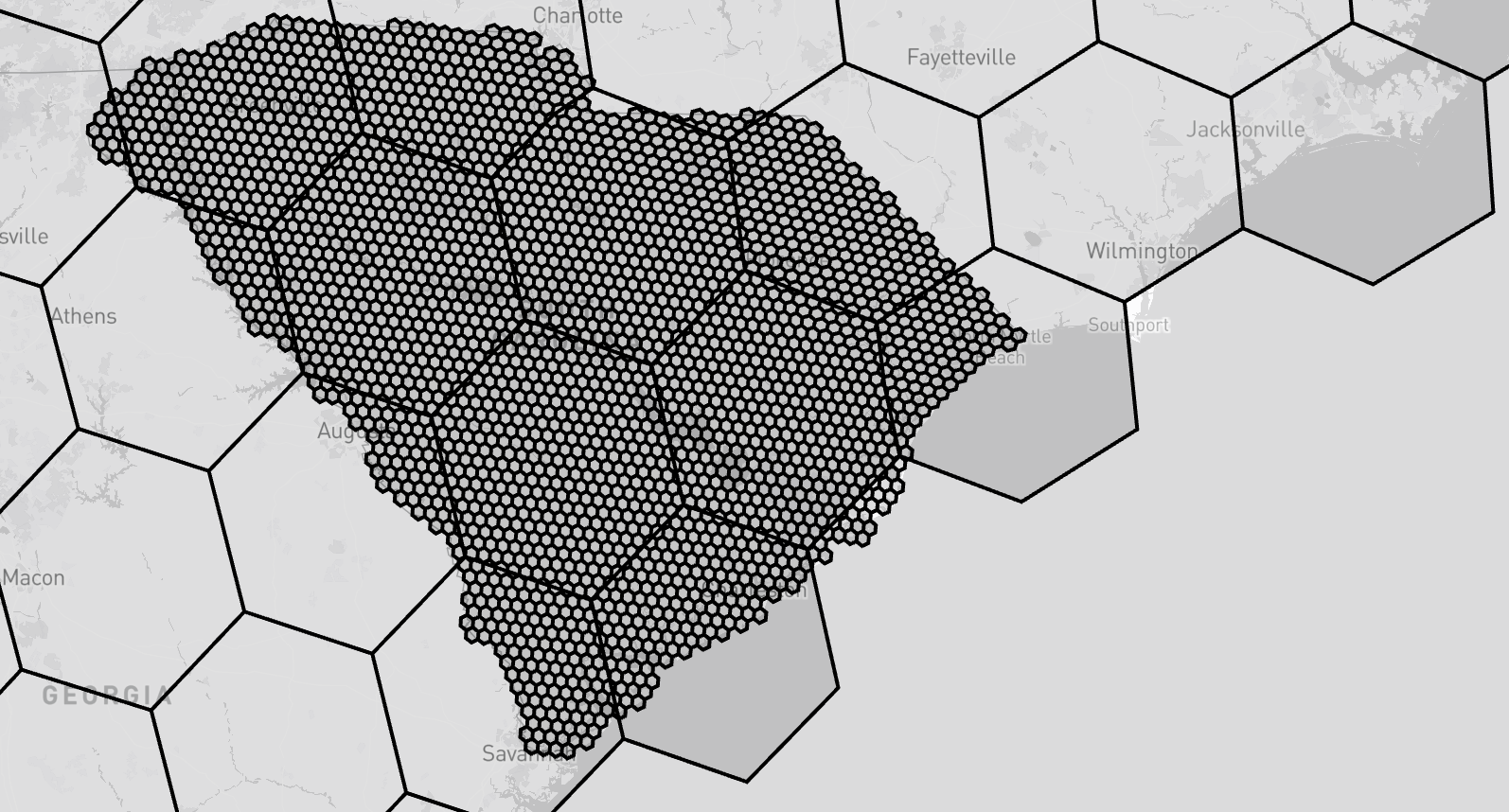
Figure 3: Edge gaps mean South Carolina isn't a perfect 100% subset of the USA

At lower resolutions (larger hexagons), the edge gaps become more pronounced. The United States set has some pretty large gaps near its edges, and a decent number of the indexes that represent South Carolina don't fall into the USA set—even though South Carolina is obviously whollycontained within the United States geographically.

There are times when I'll manually add an index to a set to cover holes like this, but that's not feasible for every set. Therefore, it becomes necessary to relax our constraint on the idea of a subset.

Enter the 93% threshold. If 93% or more of Set A's indexes appear in Set B, we call it a subset. This gives us enough wiggle room to handle edge imprecision while still maintaining a meaningful geographic relationship.

The Subset Problem: Asymmetric and Expensive

Here's where things get expensive. Subset relationships are one-way. You have to check:

• Is Set A a subset of Set B?
• Is Set B a subset of Set A?

These are completely independent checks. And you have to do this for every pair of sets.

The Performance Nightmare

Our initial implementation had these characteristics:

• Four workers processing one set against all other sets in parallel
• One set taking approximately 20 minutes to process
• 3,000 sets to process
• Total compute time of approximately 10 days

First Attempts: Making the Logic Smarter

My first instinct was to optimize the relationship detection logic itself. We made the algorithm smarter—better data structures, more efficient set operations, early termination when possible.

Did it help? Yes. Was it enough? No.

Even with optimized logic, we were still fundamentally doing too much work. The problem wasn't how we were checking relationships—it was how many relationships we were checking.

The Optimization: Containing Parent Sets

The Core Idea

Instead of comparing every set against every other set, what if we could dramatically reduce the number of sets we need to check against? Enter the containing parent.

The concept is straightforward:

1. When a set is created, find the smallest set of h3 index/s that completely contain the set to be created. We will call these the containing parents. One important thing to note is its not true that a set will be wholly contained by a single h3 index. As you down to lower resolutions you get larger and larger hexagons (h3 indexes). At some point oyu hit resolution 0 and are working with the largets hexagons that h3 supports. It is often the case that a set will not be wholly contained by a single h3 index at resolution 0. Therefore, you end up with a list of h3 indexes that completely contain the set to be created. Take for example the containing parents of the United States.

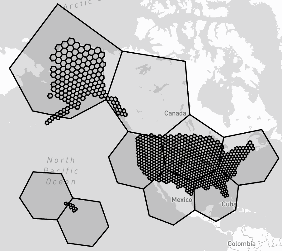
2. Store this as the set's "containing parents"
3. When computing relationships for our Set of Interest (SOI), we only check against sets that:
   • Share the same containing parents, OR
   • Has a set of containing parents that is a super set of the containing parents of the SOI

Why This Works

Geographic boundaries are naturally hierarchical. Counties are contained in states, states in countries. Cities are in counties. Parks are in cities. This hierarchical structure means that:

• A county in California will never intersect with a county in New York
• A park in Boston won't intersect with a neighborhood in Seattle
• Most geographic relationships are local—things near each other interact, distant things don't

By computing the containing parent once at set creation, we can leverage this natural hierarchy to prune the search space dramatically.

The Results: From 10 Days to 1 Day

With the containing parent optimization we were able to reduce the compute time from approximately 10 days to approximately 1 day.

Wrapping Up

The containing parent optimization transformed relationship computation from an impractical batch job into something that can be run in a reasonable amount of time. By doing a little extra work upfront and leveraging the natural hierarchy of geographic data, we reduced compute time by a significant amount.